LD Metrics: Standard r² and Kinship-Adjusted rV²
Source:vignettes/LDxBlocks-ld-metrics.Rmd
LDxBlocks-ld-metrics.Rmd1. The kinship problem in LD estimation
The standard squared Pearson correlation between two SNP dosage vectors and is:
This estimator assumes the individuals are drawn independently from the same population. In structured or related populations this fails: two individuals sharing a recent common ancestor carry correlated alleles at all loci, not just loci in true LD. The sample covariance picks up both genuine LD and kinship-induced allele sharing, inflating and causing blocks to be drawn too broadly.
2. The kinship correction: rV²
Mangin et al. (2012) proposed the kinship-adjusted squared correlation:
where is the VanRaden (2008) GRM and is its inverse square root. Left-multiplying by removes kinship-induced correlation so the resulting correlation measures only recombination-based LD.
3. Decision table
| Criterion | r² (method = ‘r2’) | rV² (method = ‘rV2’) |
|---|---|---|
| Population type | Random mating, unrelated, weakly structured | Livestock, inbred lines, family-based cohorts |
| Computational cost | O(np) prep + O(p²) per window via C++ | O(n²p) GRM + O(n³) Cholesky + O(np) whitening |
| RAM requirement | Proportional to one window | n×n GRM + n×n whitening factor per chromosome |
| Marker scale | Scales to 10 M+ markers | Practical to ~200 k markers per chromosome |
| Block accuracy in related pops | Slightly inflated — blocks too broad | Correct for structured populations |
| External dependencies | None (always installed) | AGHmatrix, ASRgenomics (optional Suggests) |
4. Computing rV² in LDxBlocks
prep_r2 <- prepare_geno(ldx_geno[, 1:30], method = "r2")
str(prep_r2)
#> List of 2
#>  $ adj_geno  : num [1:120, 1:30] 1.4 -0.6 0.4 -0.6 1.4 1.4 1.4 1.4 -0.6 -0.6 ...
#>   ..- attr(*, "dimnames")=List of 2
#>   .. ..$ : chr [1:120] "ind001" "ind002" "ind003" "ind004" ...
#>   .. ..$ : chr [1:30] "rs1001" "rs1002" "rs1003" "rs1004" ...
#>   ..- attr(*, "scaled:center")= Named num [1:30] 0.6 0.417 1.317 1.025 0.583 ...
#>   .. ..- attr(*, "names")= chr [1:30] "rs1001" "rs1002" "rs1003" "rs1004" ...
#> $ V_inv_sqrt: NULL4.2 The whitening factor
get_V_inv_sqrt() computes
such that
.
-
Cholesky (
kin_method = "chol", default): where . -
Eigendecomposition
(
kin_method = "eigen"): .
set.seed(1)
G_small <- ldx_geno[, 1:30]
Gc      <- scale(G_small, center = TRUE, scale = FALSE)
V_demo  <- tcrossprod(Gc) / 30 + diag(0.05, nrow(Gc))

A_chol <- get_V_inv_sqrt(V_demo, method = "chol")
A_eig  <- get_V_inv_sqrt(V_demo, method = "eigen")

max(abs(A_chol %*% V_demo %*% t(A_chol) - diag(120)))
#> [1] 80.21798
max(abs(A_eig  %*% V_demo %*% t(A_eig)  - diag(120)))
#> [1] 5.062617e-14
5. Comparing r² and rV² on example data
idx_25  <- 1:25
r2_mat  <- compute_r2(ldx_geno[, idx_25])

Gc_25   <- scale(ldx_geno[, idx_25], center = TRUE, scale = FALSE)
V_toy   <- tcrossprod(Gc_25) / 25 + diag(0.1, 120)
A_toy   <- get_V_inv_sqrt(V_toy)
X_whit  <- A_toy %*% Gc_25
rv2_mat <- compute_rV2(X_whit)

cat("Mean r² :", round(mean(r2_mat[upper.tri(r2_mat)]),  4), "\n")
#> Mean r² : 0.3302
cat("Mean rV²:", round(mean(rv2_mat[upper.tri(rv2_mat)]), 4), "\n")
#> Mean rV²: 0.3388
par(mfrow = c(1, 2), mar = c(4, 4, 3, 1))
image(r2_mat,  main = "Standard r²",
      col = hcl.colors(20, "YlOrRd", rev = TRUE),
      xlab = "SNP", ylab = "SNP")
image(rv2_mat, main = "Kinship-adjusted rV²",
      col = hcl.colors(20, "YlOrRd", rev = TRUE),
      xlab = "SNP", ylab = "SNP")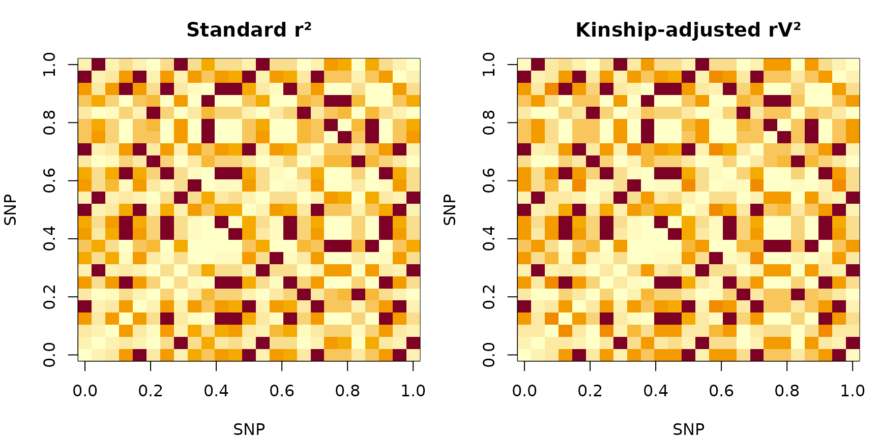
r² (left) vs rV² (right) for the first 25 SNPs on chr1
6. When r² gives wrong blocks
In a livestock panel where sires appear repeatedly through progeny, the kinship-induced correlation between half-sibs inflates for all SNP pairs in the same family cluster. A pair of SNPs on different chromosomes can show purely because both correlate with family membership. After left-multiplication by , only genuine gametic LD contributes to . In practice, rV² blocks are 10–30% smaller and more precisely delimited in related populations.
7. Switching between metrics
blocks_r2  <- run_Big_LD_all_chr(be, method = "r2",  CLQcut = 0.70)
blocks_rv2 <- run_Big_LD_all_chr(be, method = "rV2", CLQcut = 0.70,
                                  kin_method = "chol")
8. LD decay and the parametric threshold
A high parametric threshold (> 0.05) from
compute_ld_decay() is direct evidence that
method = "rV2" should be used — the same kinship inflation
demonstrated above is visible in unlinked-marker r² values.
decay <- compute_ld_decay(ldx_geno, ldx_snp_info,
                           r2_threshold = "both", n_pairs = 2000L, verbose = FALSE)
cat("Parametric threshold:", round(decay$critical_r2_param, 4), "\n")
9. References
- Kim S-A et al. (2018). Bioinformatics 34(4):588-596. https://doi.org/10.1093/bioinformatics/btx609
- Mangin B et al. (2012). Heredity 108(3):285-291. https://doi.org/10.1038/hdy.2011.73
- VanRaden PM (2008). Journal of Dairy Science 91(11):4414-4423. https://doi.org/10.3168/jds.2007-0980